|
Contributed by Sebastian Bonhoeffer; adapted for BioSym by Stefan Schafroth
Nicholson & Bailey proposed a model for host-parasitoid dynamics in the 1930s. This model describes the population of hosts and parasitoids in discrete time steps. A central characteristic of the Nicholson-Bailey model is that both populations undergo oscillations with increasing amplitude until first the host and then the parasitoid population dies out. This module first investigates the population dynamics of the simple Nicholson-Bailey model, and then extends the model to consider spatial distribution of both host and parasitoid to investigate the effect of spatial structure on stabilizing the population dynamics. We simulate the dynamics on a two-dimensional lattice (i.e. a square grid of cells).
In the 1930s Nicholson and Bailey proposed a simple discrete-time model for the population dynamics of insect hosts and their parasitoids that has since become one of the classical models of population biology. Parasitoids, such as parasitic wasps, lay eggs into their hosts and thus the completion of the parasitoid life cycle requires that their hosts be killed. Parasitoids resemble parasites as they grow inside a host, but also resemble predators in that they are obligate killers of their host.
The following concepts and methods that can be illustrated with the Nicholson-Bailey model:
The
Here and represent the densities of the host and parasitoid population at year t. R is the number of offspring of an unparasitized host surviving to the next year. Assuming random encounter between hosts and parasitoids the probability that a host escapes parasitism can be approximated by , where a is a proportionality constant. Similarly, the probability to become infected is then given by . Finally, the parameter c describes the number of parasitoids that hatch from an infected host.
The equilibrium of the Nicholson-Bailey model is obtained by setting and and is given by
and
However, this equilibrium is
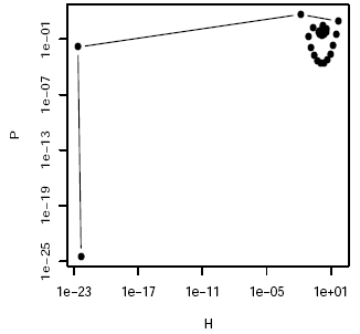
The simulation of the Nicholson-Bailey model (figure 1) shows that the dynamics are characterized by oscillations of increasing amplitude until the population crashes.
|
|
Although host-parasitoid interactions are often characterized by very strong fluctuations from year to year, unlike in the simple Nicholson-Bailey model, they typically do not lead to the complete extinction of either the host or the parasitoid. One important factor neglected in the Nicholson-Bailey model is space. Space can be neglected if the populations can be considered to be well mixed. However, this may often not be justified. Both the interactions between species and the dispersal of offspring may be local.
The Nicholson-Bailey model can be extended to incorporate space. To this end we consider a spatial grid on which the Nicholson-Bailey dynamics take place. At each site (i, j) in the grid the dynamics are (more or less) given by the simple Nicholson-Bailey model of the previous section, but in addition we allow that hosts and parasitoids disperse to all immediately neighbouring sites (with dispersal rates and ). Mathematically, the spatial model is thus given by the following equations
where the time dependence is no longer indicated by a subscript but by brackets. Here
where the sum is over all 8 neighbouring fields (i.e. (i - 1, j - 1), . . . , (i + 1, j + 1)).
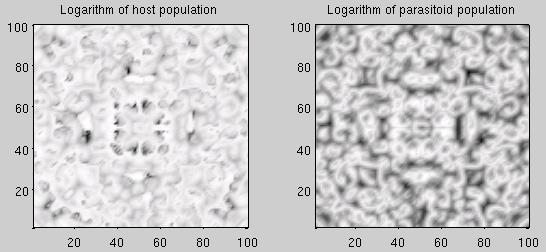
Importantly, it can be shown (see figure 2) that in the spatial Nicholson-Bailey model hosts and parasitoids can coexist indefinitely (in contrast to the non-spatial model).
|
A sample Matlab scripts that implements a two dimensional spatial Nicholson-Bailey model is provided in nb2d.m.
Eb1: Why does the simple Nicholson-Bailey model show unstable oscillations? How could it be stabilized? Try to implement realistic biological factors to achieve this. Some possible stabilizing factors are: self-limitation in the host or the parasitoid (see the module on logistic difference equation), constant immigration from the neighbourhood, sanctuary for a part of the host population, or experiment with your own ideas.
Eb2: How does the spatial dispersal rate of hosts and parasitoids affect the population dynamics of the spatial model and why? Determine the probability of coexistence or extinction for different combinations of the two dispersal rates and plot the results in a 2D plot of the parameter space (i.e. in a coordinate system with axes corresponding to the two parameters). In the regime of stable coexistence, plot the host and parasitoid densities as a function of the two parameters. (You may also experiment with changing R, a or c).
Ea1: Implement extinction in the models. Introduce a cut-off value below which the population density is set to zero. This can be done in both the simple and the spatial model. Hints for the latter: logical operations on matrices (e.g. h<cutoff) produce a matrix of logical values; multiplication with logical values behaves as if TRUE=1 and FALSE=0.
Ea2: Vary lattice size and boundary conditions, and test their effect on the probability of coexistence. How is the stable size of the global population in the spatial model related to the (unstable) equilibrium point in the non-spatial system?
Ea3: Given the instability of the system, initial conditions can greatly influence the outcome even in the spatial model. Try out different initial conditions. Hint: use the runif() function to generate random initial values for the population sizes in each cell. Alternatively, you can start the system with non-zero populations in just one or a few cells (as in Hassel et al). Investigate Exercise Eb1 with both alternatives.
Ea4: Does the order of dispersal and reproduction matter?
Ea5: What would happen if either the hosts or the parasitoids spread equally over the entire space?
Ea6: Introduce 'long-lived' parasitoids (i.e. a fraction surviving even in the absence of hosts in the lattice cell) and show how it affects the stability of the system.
Ea7: Introduce self-limitation in the host or other stabilizing factors and show how it affects the spatial dynamics.
Ea8: Measure the correlation between the dynamics at two sites as a function of their distance. How strong is the spatial correlation and how does that depend on the parameters controlling parasitoid and host dispersal? A lattice can be regarded as an infinite twodimensional surface, if the correlation length is smaller than half of the side length of the lattice. Check whether this criterion is fulfilled for the parameters that you use. Hint: measuring all pairwise correlations between the cells of the lattice may require a lot of computer time. Experiment with a small lattice first. (Note: Solving this exercise alone qualifies this module as level 2. However, it is both difficult and computationally intensive.)
Ea9: Can parasitoids facilitate the coexistence of competing hosts? Introduce two host types and either one parasitoid type affecting both hosts or two parasitoid types specialized to the two hosts. Hint: to be able to simulate the system without parasitoids, introduce logistic self-limitation in the hosts.
Difference equations: Also referred to as maps, difference equations describe the dynamics (change) of variables (e.g. the population size) in discrete time, whereas differential equations describe the dynamics in continuous time.
Unstable oscillations: Oscillations with increasing amplitudes.
Parasitoid: A lifestyle that mixes the features of true parasites and predators. Similar to parasites, parasitoids develop within their host, but the completion of their lifecycle always results in the death of the host.